Query
Expressed in SQL
First, let’s examine how this query could be expressed in SQL. If the previous data set was stored in a database table named “dailytemperatures”, the query could be expressed in the following pseudo-SQL:
SELECT dt.city, max(dt.high-dt.low)
FROM dailytemperatures dt
WHERE dt.date >= '2012-07-01' and dt.date <= '2012-07-04'
GROUP BY dt.city
Expressed as a LogicalGraph
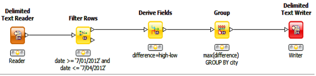
The same query also can be represented as a LogicalGraph in DataFlow:
Specifically, the processing can be accomplished by the following chain of operations, with the results of one operation feeding into the next:
1. Delimited Text Reader: This can be any DataFlow source. DataFlow supports a number of sources out of the box. In addition, it can be extended to handle new sources. (For more information about the various sources, see
Performing I/O Operations.)
3. DeriveFields: This operator is used to derive one or more new fields from existing fields in the input data. In this case, we use it to calculate the difference between the daily high and daily low. The difference is a new field, “difference”. (For more information about the DeriveFields operator, see
Using the DeriveFields Operator to Compute New Fields.)
4. Group: This operator performs aggregations over data, grouped by a specific set of fields. In this case, we use it to calculate the maximum difference, grouped by city. (For more information about the Group operator, see
Using the Group Operator to Compute Aggregations.)
5. Delimited Text Writer: This can be any DataFlow sink. DataFlow supports a number of sinks out of the box. In addition, it can be extended to handle new sinks. (For more information about various sinks, see
Performing I/O Operations.)
Corresponding Physical Graphs (Distributed)
The above LogicalGraph is then translated to a series of physical graphs. Let's assume that our run time configuration is the following:
• distributed
• parallelism=4
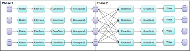
The resulting physical graphs would be:
The physical graphs for these operators are identical to the original LogicalGraph but replicated according to the parallelism setting. Specifically:
• Delimited Text Reader: There are four copies of the original reader. The input is divided into four roughly equal-sized partitions and then read by each of the copies.
• FilterRows: Parallelism is straightforward: each of the four copies independently filter their respective partitions, producing partitions that contain only those rows in the date range 07/01/2012 through 07/04/2012.
• DeriveFields: Parallelism is straightforward: each of the four copies independently computes the difference field, producing partitions that contain the original data with the additional difference field appended.
• Delimited Text Writer: Parallelism is straightforward: each of the four copies independently writes a results file.
The Group operator is also replicated per the configured parallelism setting. However, the Group operator cannot operate independently on each of the partitions. Thus a repartition is required. Specifically, the Group operator consists of the following pieces:
• Group(partial): Computes per-partition aggregations. As you will see below, this corresponds to calculating per-partition maximum temperature difference. This step is an optimization to reduce the amount of data to redistribute in the next step.
• Repartition: Per-partition aggregations must be redistributed so that rows of the same city reside in the same partition.
• Group(final): Computes overall aggregations. As you will see below, this corresponds to calculating overall maximum temperature difference.
Note: This is a somewhat simplified description of how per-partition aggregations are computed. For more information, see the example in
Writing an Aggregation.
Because a repartition is required, this causes the overall execution to be split into two phases. Between the phases, the intermediate data is staged (written to disk).
Corresponding Physical Graphs (Pseudo-distributed)
Let’s assume that our run time configuration is the following:
• pseudo-distributed
• parallelism=4
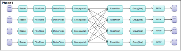
The resulting physical graphs would then be:
The physical graph for the pseudo-distributed case is nearly identical to that of the distributed case. The difference is that the pseudo-distributed graph is run in a single phase.